How to use flamegraphs for performance profiling

Learning objectives

Profiling lets you observe a live system to see where the code is spending its time. This in turn implies which application behaviors are relatively expensive (whether slow or frequently called).

Where the time is spent can shift as a result of changes to code or configuration or how users are interacting with the system. So comparing profiles under different workloads can reveal different bottlenecks. And comparing profiles of the same workload under different configurations or application versions can precisely identify performance regressions.

Understanding what parts of the code are expensive can help guide optimization and tuning efforts, and sometimes it uncovers unexpected inefficiencies.

In this tutorial, you will learn how to:

• Generate flamegraphs using sampling profilers such as perf.
• Interpret the shape and structure of flamegraphs to find which code paths are hot.
• Identify what important behaviors are implicitly omitted by profilers that only sample processes while they are actively running on a CPU.

For troubleshooting incomplete or broken profiling results, it is helpful but not required to have a basic understanding of how compilers and linkers work. The essentials will be covered in this tutorial.

Quick tour of a flamegraph

As a quick preview of what we will be learning, here is an example flamegraph with doodles highlighting some noteworthy parts.

It may look complex at first, but don’t be intimidated. By the end of this tutorial, you will know how to read the shape and structure of the graph to identify which code paths consume relatively large amounts of CPU time.

Interactive SVG image — Open this link in its own browser tab to zoom in and see full function names.

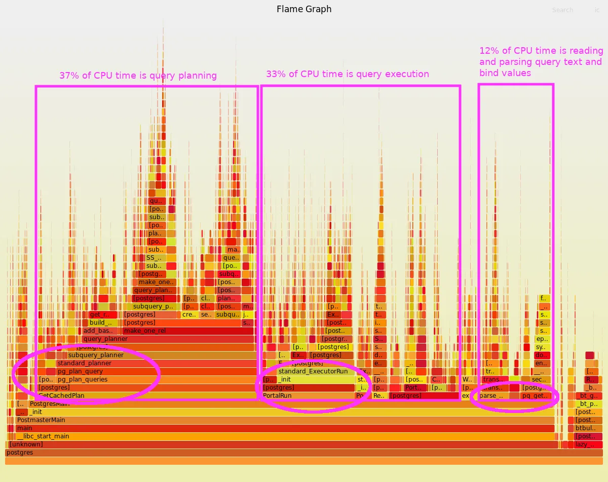
What am I looking at?

The above flamegraph shows where CPU time is being spent by our primary production Postgres database. For now, don’t worry about the details of this particular graph; just get familiar with its appearance and layout.

We will go through this in more detail later, but as a preview, here are some key points for interpreting a flamegraph:

• Each colored cell in the graph represents a function that was called by one of the processes being profiled.
• As a whole, the graph represents a large collection of stack traces.
• Each of those stack traces records the chain of function calls that lead up to whatever function was actively running on the CPU at that moment in time.
• The function call chain is read from the bottom up.
  • For example, main calls PostmasterMain, which calls _init, which calls PostgresMain.
  • The tips at the top of each tower show the function that was running on the CPU during one or more of the stack traces, and all the functions directly below it are its ancestors in its call chain.
• Collectively, the graph shows which call chains were seen the most often: the wider the function’s colored cell, the more often the call chain up to that point was seen by the profiler.

Tip: You do not have to know what every function does. A little context goes a long way.

For example:

• We know that Postgres is a SQL database.
• Like most databases, when a client sends it a query, before it can run that query, it must make a plan (e.g. choose which indexes would be most efficient, what order to join tables, etc.).
• Without even looking at the source code, when we notice that the graph is showing us function pg_plan_query calling standard_planner calling subquery_planner, we can reasonably infer that this is part of Postgres’ query planner code path.

Similarly:

• We know that Postgres must also run those queries after it chooses an execution plan.
• When we notice the graph showing us a wide cell for function PortalRun that spends most of its time calling standard_ExecutorRun, we can reasonably infer that this is a common code path for executing a query.

Conversely, if you did not already know that relational databases like Postgres have query planners, exploring that call chain in the graph would lead you to discover that query planning is a significant activity of the database.

Exploring the call chains in a flamegraph can be a way to learn interesting internal behaviors of even programs that you know very little about. It shows which components are interacting for your workload, which lets you focus your exploration on those particular code paths that matter in your environment.

What is this telling me?

Perhaps surprisingly, one of the stories this graph tells is that the way we currently use Postgres, it spends a larger proportion of its CPU time parsing and planning queries than it does actually running them.

This relatively high overhead is not obvious from looking at just query latency statistics, and it is not typical of many other Postgres workloads. CPU profiling has given us a novel perspective on the essential performance question “Where was the time spent?” — a perspective that is specific to our workload, configuration, and environment.

What is causing that?

Note: Skip this section unless you are curious about why the overhead shown above is occurring. This tangent is not about flamegraphs; it is about how we use Postgres at GitLab.

Why is our workload forcing Postgres to spend so much time in query planning?

The high proportion of time spent planning queries versus running them may be a side effect of the database clients not using prepared statements. They connect to Postgres through a connection pooler (PgBouncer) that is configured to lease a physical db session to the client for the shortest possible duration (1 transaction). This prevents clients from using prepared statements across transaction boundaries.

Consequently, clients must frequently resend the same query text, and Postgres must parse and plan it each time as though it was new.

Each individual query still completes quickly — when the queries are simple, planning is quick. But proportionally the CPU overhead is large, so at a high query rate, it adds up to a lot of CPU time.

It could save perhaps as much as 30% CPU time if clients were able to use long-lived prepared statements to parse and plan each query once and then skip the overhead during subsequent runs. A future release of Postgres may make that possible, but currently each db session has its own private pool of prepared statements and cached query plans.

How to make flamegraphs from perf profiles

Linux’s perf tool supports several different profiling techniques. Here we will focus on just one use case:

Capture a timer-based series of stack traces from processes actively running on a CPU.

Timer-based profiling is arguably the most common use-case, and mastering it gives you a good foundation for more advanced cases (e.g. profiling which code paths make calls to a specific function).

The easy way: Helper scripts

A set of convenience scripts that is available on all of GitLab.com’s Chef-managed hosts.

These helper scripts make it easy to quickly capture a perf profile and generate a flamegraph with a minimum of arguments.

• They run for 60 seconds capturing stack traces at a sampling rate of 99 times per second.
• When finished, they generate a flamegraph (which you can download and open in your browser), along with the raw stack traces as a text file.
• Depending on which script you use, it will capture one, some, or all running processes on the host.

Here are the scripts:

• perf_flamegraph_for_all_running_processes.sh takes no arguments.
  • This is the most general-purpose script.
  • It captures the whole host’s activity. It essentially runs with no filters, so whatever processes are running on the CPU will be sampled by the profiler.
  • Use it when you do not have time to be more specific about what to capture or when you need to capture multiple processes.
  • When you view the flamegraph, you can interactively zoom in to see only the processes you care about.
• perf_flamegraph_for_pid.sh [pid_to_capture] takes 1 argument: the PID of the process to capture.
  • This is convenient when you want to profile a single-process application like Redis or HAProxy.
  • If you want to capture multiple PIDs, you can give it a comma-delimited PID list, but it may be simpler to instead just capture all running processes.
  • If the PID you specified forks any child processes while perf is running, they will implicitly be profiled as well, but any pre-existing child processes will not automatically inherit profiling.
• perf_flamegraph_for_user.sh [username_to_capture] takes 1 argument: the username or UID of a Unix account whose processes you want to capture.
  • This is convenient when a multi-process application runs as a specific user, such as gitlab-psql on our patroni-XX hosts or git on our web-XX hosts.
  • Caveat: This may fail to start if the user runs extremely short-lived processes that disappear during perf startup, before they can be instrumented. If this happens, consider instead using perf_flamegraph_for_all_running_processes.sh.

Example: Profile the redis-server process on the primary redis host.

$ ssh redis-03-db-gprd.c.gitlab-production.internal

$ pgrep -a 'redis-server'
2997 /opt/gitlab/embedded/bin/redis-server 0.0.0.0:6379

$ perf_flamegraph_for_pid.sh 2997
Starting capture.
[ perf record: Woken up 1 times to write data ]
[ perf record: Captured and wrote 0.335 MB perf.data (1823 samples) ]
Flamegraph:       /tmp/perf-record-results.VIZtuZzA/redis-03-db-gprd.20200618_153650_UTC.pid_2997.flamegraph.svg
Raw stack traces: /tmp/perf-record-results.VIZtuZzA/redis-03-db-gprd.20200618_153650_UTC.pid_2997.perf-script.txt

You can then download the flamegraph to your workstation and open it in your (javascript-enabled) web browser to explore the results.

scp -p redis-03-db-gprd.c.gitlab-production.internal:/tmp/perf-record-results.VIZtuZzA/redis-03-db-gprd.20200618_153650_UTC.pid_2997.flamegraph.svg /tmp/

firefox /tmp/redis-03-db-gprd.20200618_153650_UTC.pid_2997.flamegraph.svg

Interactive SVG image

If you wish, you can also review the individual stack traces in the *.perf-script.txt output file: perf-script.txt.gz

We will talk more about stack traces shortly. For now just be aware that this is available if you need it.

Once you are comfortable using these helper scripts, you may later be interested in customizing what gets captured or how it gets rendered. A brief introduction to such tricks is included at the end of this tutorial: Bonus: Custom capture using perf record

How to interpret flamegraphs for profiling where CPU time is spent

Background: What is a stack trace?

When a program is run, it begins at a well-defined entry point. (For example, in C programs, the entry point is a function named “main”.) That function typically calls other functions which perform specific tasks and then return control to the caller. At any point in time, a thread will be executing one particular function whose called-by ancestry can be traced all the way back to the program’s entry point.

Tracing the ancestry of the currently executing function is called generating a “stack trace”.

Each function call in that ancestry is called a “stack frame”.

Generating a stack trace effectively means figuring out the name of the function associated with each stack frame.

Recovering the names of the functions for compiled software can be surprisingly hard. In pursuit of other efficiencies, compilers often make tracing difficult. Usually this shows up as missing stack frames or unknown function names. Later we will review a few examples, but for now, just be aware that these deficiencies can occur. Remedies such as resolving debug symbols may or may not be straightforward depending on how the software was built.

Example stack trace

Here is an example stack trace, showing a Redis thread doing a key lookup. For now, ignore the 1st and 3rd columns; just look at the middle column which shows the function name for each stack frame.

           2c63d  dictFind                (/opt/gitlab/embedded/bin/redis-server)
           47c1d  getExpire               (/opt/gitlab/embedded/bin/redis-server)
           47d4e  keyIsExpired            (/opt/gitlab/embedded/bin/redis-server)
           48a92  expireIfNeeded          (/opt/gitlab/embedded/bin/redis-server)
           48b2b  lookupKeyReadWithFlags  (/opt/gitlab/embedded/bin/redis-server)
           48bdc  lookupKeyReadOrReply    (/opt/gitlab/embedded/bin/redis-server)
           56510  getGenericCommand       (/opt/gitlab/embedded/bin/redis-server)
           306ee  call                    (/opt/gitlab/embedded/bin/redis-server)
           30dd0  processCommand          (/opt/gitlab/embedded/bin/redis-server)
           41b65  processInputBuffer      (/opt/gitlab/embedded/bin/redis-server)
           29f24  aeProcessEvents         (/opt/gitlab/embedded/bin/redis-server)
           2a253  aeMain                  (/opt/gitlab/embedded/bin/redis-server)
           26bc9  main                    (/opt/gitlab/embedded/bin/redis-server)
           20830  __libc_start_main       (/lib/x86_64-linux-gnu/libc-2.23.so)
6c3e258d4c544155  [unknown]               ([unknown])

The top stack frame shows the currently executing function (dictFind), and the bottom few stack frames show the generic entry point for the program. As mentioned earlier, all C programs start with a function named main. The bottom 2 frames in this stack trace are generic, and the main frame is the earliest part of the stack that is specific to the program we are tracing (redis-server).

Reading up from the bottom, we see Redis’s main function makes a call to aeMain, which calls aeProcessEvents, which calls processInputBuffer, etc. Even without reviewing the redis source code, we can infer that aeProcessEvents is part of an event handler loop, and processInputBuffer is part of an event it is handling.

Looking further up the stack, we see processCommand -> call -> getGenericComand. Again, without looking at the redis source code, we can already infer what this means, with just a little bit of background on what Redis is: Redis is a key-value store that expects clients to send commands like GET, SET, DEL that operate on the keys it stores. So this part of the stack tells us that this redis thread was performing a GET command. We cannot see from the stack trace what specific key it was operating on, but we can see what part of the GET command was running at the time we captured this stack trace.

Looking further up at the remaining stack frames, we can infer that redis was checking to see if the requested key is expired before responding to the client’s GET command. Redis supports tagging any key with a finite time-to-live. The expireIfNeeded function checks whether or not this key has exceeded its time-to-live.

So this one stack trace shows us what this redis thread was doing at a single moment in time. How is this useful?

A single stack trace by itself can be useful if it was associated with a special event (e.g. a crash). But for performance analysis, we usually want to capture a bunch of stack traces and aggregate them together. This aggregation shows us which call chains occur most often, which in turn implies that is where the most time is spent. There are some caveats that we will review later, but for now let’s look at an example of how sampling stack traces roughly every 10 milliseconds for 30 seconds can give us a picture of how our process threads are spending their CPU time.

How are stack traces aggregated into a flamegraph?

The example stack trace we examined above was a random pick from the 637 stack traces sampled by this command:

$ pgrep -a -f 'redis-server'
2997 /opt/gitlab/embedded/bin/redis-server 0.0.0.0:6379



$ sudo perf record --freq 99 -g --pid 2997 -- sleep 30
[ perf record: Woken up 1 times to write data ]
[ perf record: Captured and wrote 0.125 MB perf.data (637 samples) ]



$ sudo perf script --header | gzip > redis_stack_traces.out.gz

To aggregate those 637 stack traces into a flamegraph, we can run:

git clone --quiet https://github.com/brendangregg/FlameGraph.git

zcat redis_stack_traces.out.gz | ./FlameGraph/stackcollapse-perf.pl | ./FlameGraph/flamegraph.pl > redis-server.svg

The stackcollapse-perf.pl script folds the perf-script output into 1 line per stack, with a count of the number of times each stack was seen. Then flamegraph.pl renders this into an SVG image.

View as an interactive SVG image

Flamegraphs in SVG format are interactive

When viewed in a Javascript-capable browser, the SVG image supports interactive exploration:

• Mouseover any frame to see: the full function name, the number of times that function was called in this call chain, and the percentage out of all sampled stacks that this function and its ancestors were seen.
  • Example: The all virtual frame is included in 100% of the 637 stack traces. The beforeSleep frame is included in 38.5% (245 out of 637 stack traces).
• Zoom into any portion of the graph by clicking any frame to make it fit the full width of the display. This lets you more easily see the names and shape of a portion of the call graph.
  • Example: Click the frame for vfs_write in the wide righthand portion of the flamegraph. Then to zoom back out, click either “Reset Zoom” or the bottom frame labeled all.
• Search for function names, to highlight all occurrences of that string.
  • Example: Search for expireIfNeeded. Several different call chains include this function, and they are now all highlighted in magenta. The bottom righthand corner of the flamegraph shows that a total of 6.8% of stack traces include that frame somewhere.

In flamegraphs, plateaus are relevant, spikes are not

When interpreting flamegraphs, the main thing to remember is: width matters, height does not.

The width of any stack frame in the flamegraph represents the number of sampled events that included the exact same chain of function calls leading up to that point.

If the event sampling strategy was timer-based sampling (e.g. capture stack traces 99 times per second if the process is currently running on CPU), then the more often you see a common series of function calls, the more CPU time was spent there. Consequently, any function appearing in a wide frame was part of a frequently active call chain.

For example, in the above flamegraph, redis-server spent 47% of its CPU time in aeProcessEvents (where client commands get processed), but because that frame was almost never at the top of the stack, we know that very little CPU time was spent in that function itself. Mostly aeProcessEvents calls other helper functions to perform work, such as processInputBuffer, readQueryFromClient, and the read syscall to read bytes from TCP sockets.

Overall, we can see from this flamegraph that redis-server spends a significant amount of its CPU time doing network I/O.

Also, ignore the colors. By default, they are randomized from a red/orange color pallette, just to show at a glance which cells are wide. Optionally, it is possible to choose other more meaningful color schemes, such as:

• Choose the color by function name, to more easily see multiple occurrences of functions that appear in multiple call chains.
• Use a different hue for kernel functions than userspace functions, so syscalls are easier to see.

Common profiling gotchas

When profiling with perf, there are a few things to be aware of, and issues you might run into.

• Off-CPU time: The most common type of profiling will tell you about time spent running on the CPU. However, it may also be interesting to understand why a process is being de-scheduled (e.g. IO and other blocking syscalls, waiting for a wake-up event, etc.). For this purpose you can perform an off-CPU analysis.
• Incomplete/incorrect stack traces: To produce a stack trace, perf has to “unwind” the stack, finding the address of each stack frame’s next instruction. To do this stack walk, perf by default relies on frame pointers. However, for largely historical reasons, compilers often try to use an optimization technique that opportunistically omits frame pointers. This can cause perf to produce bogus call graphs. This kind of breakage is obvious when it occurs. As a work-around, you can tell perf to use an alternative method for unwinding stacks (e.g. --call-graph=dwarf). See the manpage for perf record for more details. Alternately, if you happen to be able to customize the build procedure for the binary you want to trace, you can explicitly request that the compiler use frame pointers (e.g. add CFLAGS=-fno-omit-frame-pointer when the compiling the binary you are analyzing). Doing so may fix framepointer-based stack unwind (for perf and other similar profilers).
• Missing function names: Another thing that perf needs is symbols. If symbols were stripped from the binary as part of the build procedure, then perf cannot translate addresses into function names. Sometimes the build process will produce a separate package containing debug info, including symbols, and installing that supplemental package (e.g. -dbg or -dbgsym suffix) will provide the missing symbols. Alternately, if you control the build procedure for the binary you want to trace, you can disable stripping symbols. This is standard practice for most of GitLab’s build pipelines, so typically the binaries shipped by GitLab do have all of their debug symbols.
• Catching or excluding rare outlier events: A sampling profiler will not catch examples of every executed code path. Rare events may not show up in profiles. If you need to capture rare events involving a certain code path or need to audit every code executed code path that leads to a certain function, you can use perf for tracing specific events via kprobes or uprobes. Rather than sampling based on a timer, this use-case captures data (e.g. increments a counter or saves a stack trace) every time that instrumented function call occurs. This may incur a noticeable overhead for very frequently executed functions, so use this approach with caution. If the function you want to trace is called a million times per second, consider if there are other functions that could answer the same question, and if you must use high frequency instrumentation, keep the tracing brief.

Bonus: Custom capture using perf record

Without using the convenience scripts described above, the steps to make a flamegraph of all on-CPU activity for a host typically looks like this:

$ sudo perf record --freq 99 -g --all-cpus -- sleep 60



$ sudo perf script --header > perf-script.txt


$ git clone --quiet https://github.com/brendangregg/FlameGraph.git


$ ./FlameGraph/stackcollapse-perf.pl < perf-script.txt > perf-script.folded.txt


$ ./FlameGraph/flamegraph.pl < perf-script.folded.txt > flamegraph.svg

Or more concisely:

git clone --quiet https://github.com/brendangregg/FlameGraph.git && export PATH=./FlameGraph:$PATH
sudo perf record --freq 99 -g --all-cpus -- sleep 60
sudo perf script --header | tee perf-script.txt | stackcollapse-perf.pl | flamegraph.pl > flamegraph.svg

You may still wish to use a variation of the above procedure if you need to customize some aspect of the capture or post-processing.

The next sections walk through a few examples.

Show only stacks that match a regexp

As an optional post-processing step, before feeding the folded stack traces into flamegraph.pl, you can grep it to include only the stack traces from a particular process name or that include a call to a particular function name. For example, if you only want to see call chains that include a write syscall (i.e. writes to a file or a network socket), you can do this:

cat perf-script.folded.txt | grep 'vfs_write' | ./FlameGraph/flamegraph.pl > flamegraph.svg

Capture a larger sample

Sometimes you may need more profiling data. Maybe there are relatively rare call paths don’t reliably get caught by the default sampling rate and duration. To capture more data (i.e. sample more stack traces), you can either:

• Increase the duration of the capture.
• Increase the sampling rate per second.

When practical, prefer a longer duration rather than a higher sampling frequency. A higher sampling rate adds proportionally more overhead to the processes being traced, but any of the recommended rates (49, 99, 497) should be fine for almost any workload.

To profile PID 1234 for a longer duration than 60 seconds:

$ sudo perf record --freq 99 -g --pid 1234 -- sleep 300

To profile PID 1234 at a higher sampling frequency for a shorter duration:

$ sudo perf record --freq 497 -g --pid 1234 -- sleep 30

After running perf record, you can generate a flamegraph using the same post-processing steps shown above (starting with the perf script command).

sudo perf script --header | tee perf-script.txt | stackcollapse-perf.pl | flamegraph.pl > flamegraph.svg

Tips for choosing a sampling rate

TLDR: Pick one of these safe sampling rates: 49 Hz, 99 Hz, or 497 Hz

Here’s why:

• A slightly off-center rate reduces the risk of accidentally synchronizing the capture interval with some periodic behavior of the process being observed — which would bias your samples and produce misleading profiling results.
• Keeping it close to a round number makes it easy to mentally estimate the expected event count: 99 HZ 8 CPUs 10 seconds =~ 8000 events
• These rates all have low overhead, and hence a low risk of noticeably affect the behavior or performance of the processes being traced.

Profiling costs some CPU time per event. In our case, the per event overhead of capturing the kernel and userspace stack costs roughly 1.1 microseconds (as benchmarked on a staging host while tracing a CPU-bound process).

With the timer-based stack profiling discussed above, the sampling rate is the biggest factor affecting the cumulative overhead. For example:

99 HZ (events/CPU) * 32 CPUs * 60 seconds duration * 1 microsecond/event overhead
  = 192000 microseconds of CPU time
  = 0.2 seconds of CPU time overhead spread evenly across 60 seconds and 32 CPUs

Even a single-threaded CPU-bound application can tolerate a 497 Hz sampling rate. That rate would cost the application 0.05% of its CPU time: Sampling 1 CPU at a rate of 497 times per second with an overhead of 1 microsecond per sampling event costs a total of 0.5 CPU milliseconds per wallclock second (0.05% overhead for a CPU-bound process).

Capturing events without a timer

Capturing a profile by using a periodic timer to collect samples at a regular interval usually gives a good overview of the traced processes’ behavior.

Sometimes, to dig deeper into a specific behavior, you may instead want to capture a stack trace any time the process calls a specific function or tracepoint.

Be cautious of the overhead! With timer-based profiling, the event rate is directly controlled by you, but when profiling events like a function call, the application’s behavior and workload controls the event rate.

As shown below, you can preview the event rate with a cheap counter before running the somewhat more expensive stack profiling.

$ sudo perf list | grep 'random'
  ...
  random:urandom_read                                [Tracepoint event]
  ...
  syscalls:sys_enter_getrandom                       [Tracepoint event]
  ...


$ sudo perf stat --event random:urandom_read --event syscalls:sys_enter_getrandom --all-cpus -- sleep 10


$ sudo perf record --event random:urandom_read --all-cpus -g -- sleep 10

Gotcha: Some event types ignore perf record --count N

Although perf record provides an option to sample only 1 out of N events (--count 1000 to capture 1 in 1000 events), that mechanism is silently ignored by some event types (e.g. software events implement it, but tracepoints and kprobes ignore it). If you want to instrument a high-frequency event using a kprobe or tracepoint, you cannot use --count N to downsample and reduce overhead.

Example:

When capturing tracepoint sched:sched_wakeup, even though we specify --count 1000, perf-record still captures all events. The demo below shows the same event count (178 events) as seen by both perf stat and perf record --count 1000. The --count 1000 was ignored for this tracepoint-type event, but it is honored by software-type events like page-faults.

Script:

$ cat show_perf_record_silently_ignores_count_option_for_tracepoint_events.sh
#!/bin/bash

echo "Starting target process"
dd if=/dev/zero of=/dev/null bs=1c count=10M &
TARGET_PID=$!

echo "Starting perf-record"
sudo perf record --pid $TARGET_PID -g -e 'sched:sched_wakeup' --count 100 &

echo "Starting perf-stat"
sudo perf stat --pid $TARGET_PID -e 'sched:sched_wakeup' &

echo "Waiting for all processes to exit"
wait

echo "Done"

Output:

$ ./show_perf_record_silently_ignores_count_option_for_tracepoint_events.sh
...
[ perf record: Captured and wrote 0.071 MB perf.data (178 samples) ]
...
 Performance counter stats for process id '5862':

               178      sched:sched_wakeup
...

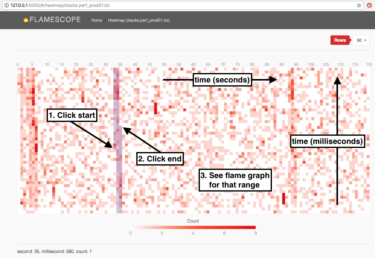
Bonus: Exploring subsets of a timeline with Flamescope

The perf-script output can be downloaded to your laptop and loaded into Flamescope, where you can more interactively explore the data you captured:

• visualize what points in the timeline had more on-CPU activity (i.e. more stack traces collected per second)
• select any portion of the timeline and generate a flamegraph for just that timespan
• directly compare two flamegraphs, somewhat like a diff for visualizing which functions were more or less prominently on-CPU during timespan A versus timespan B

To use Flamescope locally, build and run it in a docker container, and copy the perf-script files into a directory that you expose to that container:

$ git clone https://github.com/Netflix/flamescope.git
$ cd flamescope/
$ docker build -t flamescope .


$ mkdir /tmp/profiles
$ docker run --rm -it -v /tmp/profiles/:/profiles:ro -p 5000:5000 flamescope


$ cp -pi perf-script.txt.gz /tmp/profiles/



$ firefox http://0.0.0.0:5000/

Another tool that can provide ad-hoc flamegraphs and includes a time dimension is speedscope.

Learn more

Continuous profiling

In addition to the ad hoc profiling covered here, some of the GitLab components support continuous profiling.

These profiles can be accessed in the GCP Cloud Profiler.

More about perf tool

The perf tool does much more than just stack profiling. It is a versatile Linux-specific performance analysis tool, primarily used for counting or sampling events from the kernel or hardware. It can also instrument events from userspace if certain dependencies are satisfied.

Many of its use-cases overlap with BPF-based instrumentation. BPF programs typically use the kernel’s perf_events infrastructure, and perf itself can attach a BPF program to a perf_event.

Brendan Gregg’s Perf Tutorial provides a rich collection of reference material, including:

• a long annotated list of perf one-liners
• essential background why it is sometimes challenging to reassociate function names with stack frames
• summary of the different types of events that can be instrumented
• examples of using perf to answer several very different kinds of questions about system performance

kernel.org’s wiki on perf provides many more details and explained examples than perf’s already detailed manpages. In particular, it’s Tutorial includes a wealth of advice on how to use perf, interpret its sometimes opaque output, and troubleshoot errors.